

XLOOKUP in Google Sheets finds a value in one range and returns matching data from another. The lookup column doesn't need to sit to the left of the result, the way it does with VLOOKUP. I've replaced most of my old VLOOKUP formulas with it, because the result can sit anywhere.
Here's the step-by-step, plus the mistakes that produce an #N/A error. At the end, a note on when relying on XLOOKUP is a sign your spreadsheet has outgrown what it's built for.
What is XLOOKUP?
XLOOKUP is a Google Sheets function that takes up to six arguments. The first three are required: what you're searching for, where to search, and where to pull the answer from.
The other three are optional, and they're where most of the power sits: what to show when nothing matches, how strict the match has to be, and which end of the range to start from. The rest of this guide walks through all six.
What you'll need before starting
Prerequisites:
- A Google Sheet with at least two ranges you want to match up, like an order list and a customer list.
- Basic comfort with the idea of looking up one value based on another.
- No paid account or add-on required.
Time required: 3 to 7 minutes for a basic lookup, 10 to 15 minutes if you're adding fallback values or match options.
How to use XLOOKUP in Google Sheets: step-by-step
Step 1: Identify what you're searching for and where
Decide on the value you're looking up and the range that contains it. If you're pulling a customer's email based on an order's customer ID, the search value is the customer ID. The lookup range is the column of customer IDs in your customer list.
Step 2: Write the basic formula
The core syntax is:
=XLOOKUP(search_key, lookup_range, result_range)
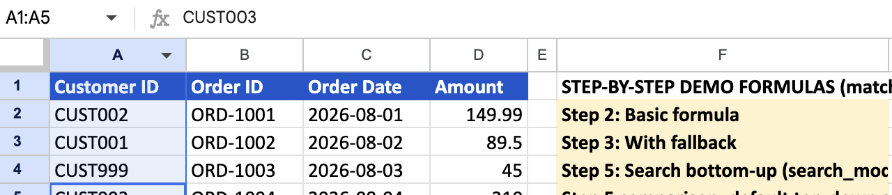
For the order-to-customer example, with the order's customer ID in A2, the customer list's IDs in Sheet2!A:A, and emails in Sheet2!C:C:
=XLOOKUP(A2, Sheet2!A:A, Sheet2!C:C)
Pro tip: The lookup range and result range don't need to be next to each other. You can search a column on the far left of a sheet and return a result from a column on the far right. The result can even come from a completely different sheet.

Step 3: Add a fallback for no match
By default, XLOOKUP returns #N/A when it can't find a match. Add a fourth argument to show something friendlier instead:
=XLOOKUP(A2, Sheet2!A:A, Sheet2!C:C, "Not found")
This replaces the old habit of wrapping a lookup in IFERROR just to catch a missing value.

Step 4: Choose a match mode if exact matching isn't enough
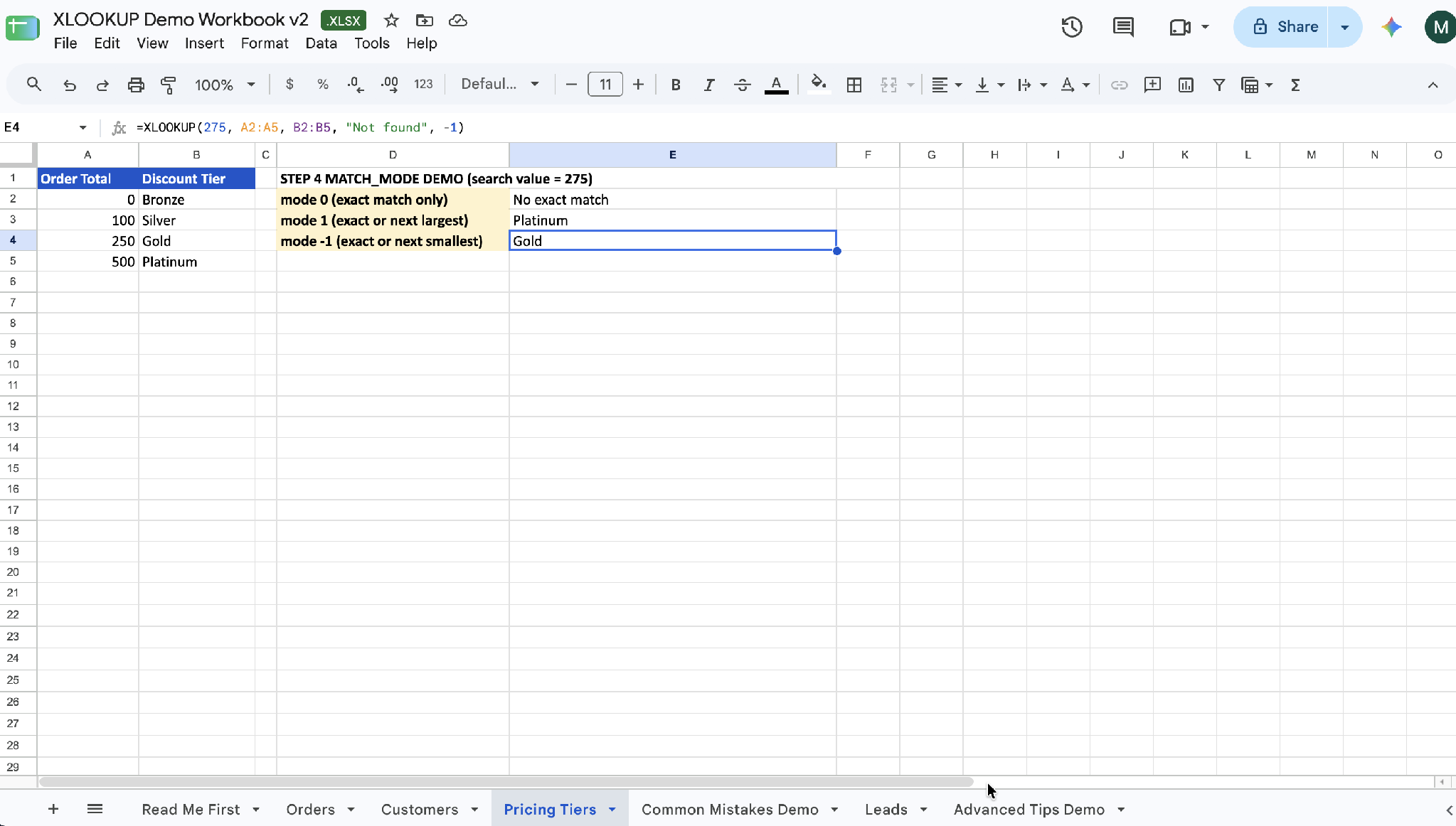
A fifth argument controls how strict the match is. The default (0) requires an exact match. Setting it to -1 finds an exact match or the next smallest value; 1 finds an exact match or the next largest value; and 2 enables wildcard matching.
=XLOOKUP(A2, Sheet2!A:A, Sheet2!C:C, "Not found", 1)
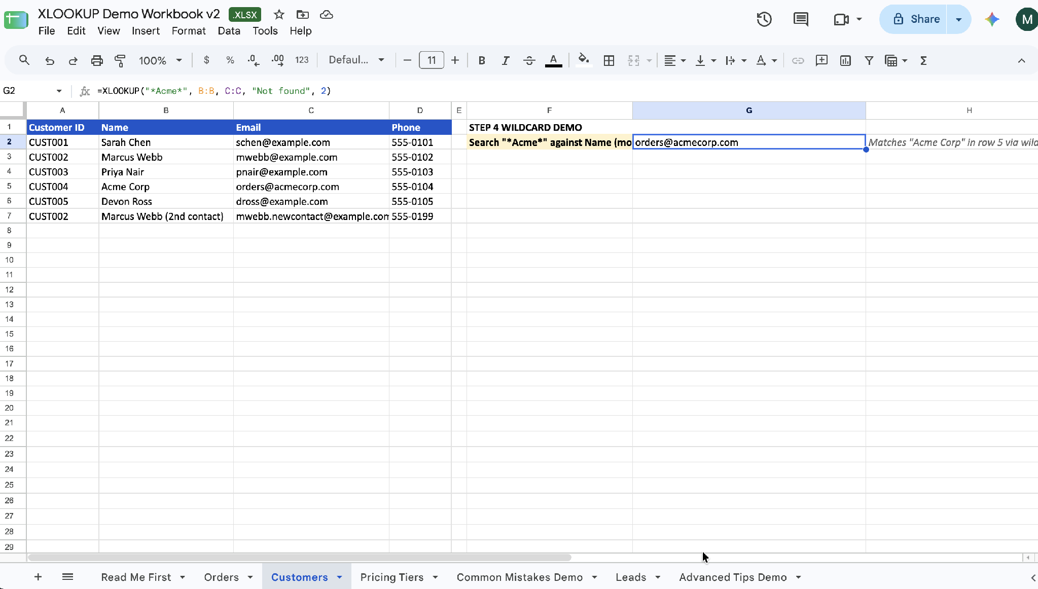
Pro tip: Wildcard matching (mode 2) is useful when you're searching for a partial string, like matching "Acme" against a lookup value stored as "Acme Corp."
Step 5: Search from the bottom up if you need the last match
A sixth argument controls search direction. The default (1) searches top to bottom and returns the first match. Setting it to -1 searches bottom to top instead, which is useful when a value appears more than once and you want the most recent entry.
Two more options run a faster binary search on a range that is already sorted. Use 2 when the range runs smallest to largest, and -2 when it runs largest to smallest. Pick the wrong one and the formula returns a wrong answer instead of an error.
=XLOOKUP(A2, Sheet2!A:A, Sheet2!C:C, "Not found", 0, -1)

Step 6: Return more than one column if needed
If the result range spans multiple columns instead of one, XLOOKUP returns all of them at once, spilling the results across adjacent cells. This can replace several separate lookup formulas with one.
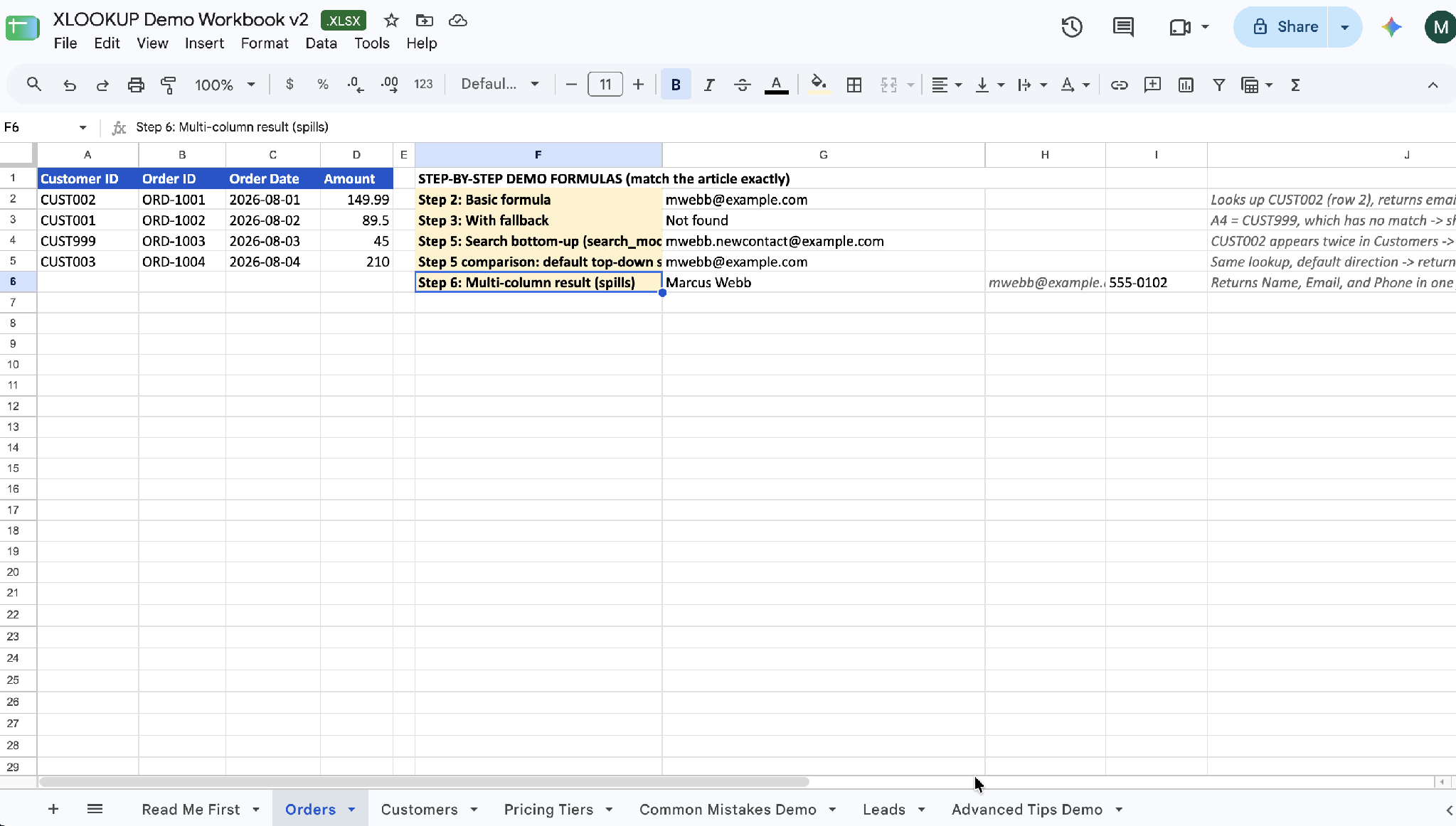
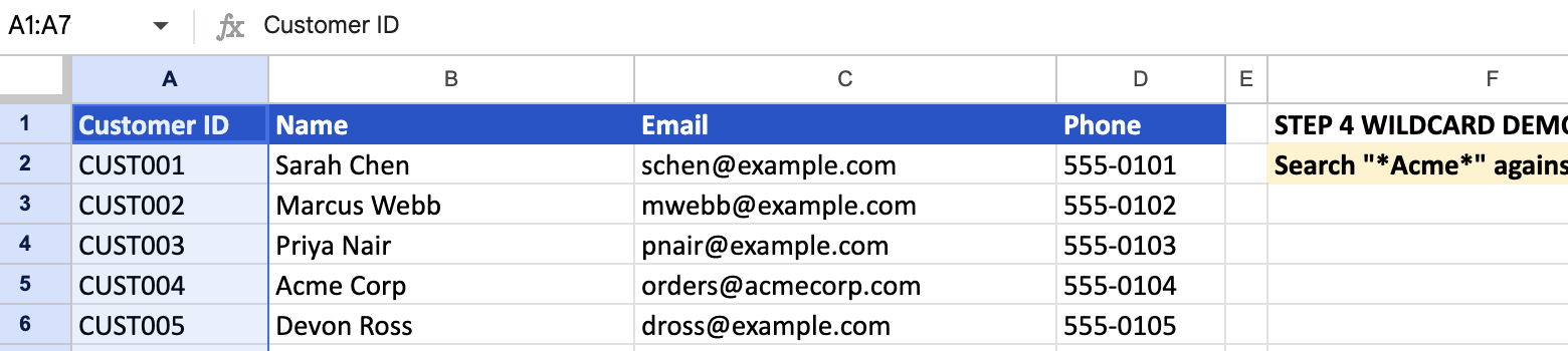
With the customer list's email in column C and phone number in column D:
=XLOOKUP(A2, Sheet2!A:A, Sheet2!C:D)
For customer ID CUST002, this spills mwebb@example.com into the first cell and 555-0102 into the one beside it, both from a single formula.
Common mistakes to avoid
Five things that trip up an XLOOKUP formula:
- Mismatched range sizes: The lookup range and result range must be the same length. A mismatch produces an #N/A error.
- Swapping the lookup and result ranges: Since the two ranges are separate arguments, not one table with a column index, it's easy to put them in the wrong order. Double-check which range you're searching and which you're returning from.
- Skipping the fallback value: Leaving out the fourth argument means a missing match shows as a raw #N/A error instead of something readable.
- Forgetting the match mode isn't automatic: An exact match is the default. If your data has slight variations or you expect an approximate match, you need to set the fifth argument explicitly.
- Capping the lookup range at today's last row: An open-ended lookup range like A:A covers the whole column, including rows added later. A fixed range like A2:A100 silently stops covering new rows past 100, the kind of fragility that eventually pushes some teams toward a full Google Sheets alternative.


Advanced tips
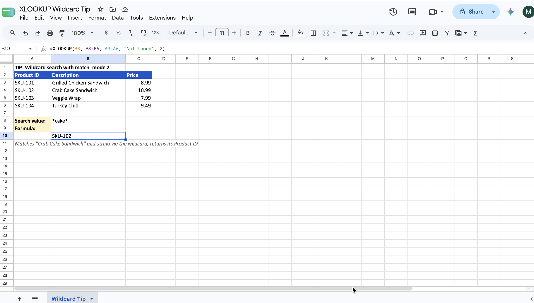
Use a wildcard for a partial match: Set the fifth argument (match_mode) to 2, then use an asterisk in the search key to match any text around it. "*cake*" finds a product with "cake" anywhere in its name. Google Sheets supports three wildcards here. Use * to match any run of characters, ? to match exactly one, and ~ when you need to search for a literal * or ?.
Combine with IF for conditional lookups: Wrapping XLOOKUP in an IF statement lets you run a different lookup depending on a condition. One example is checking one list for existing customers and a different list for new leads.

Use it across sheets and files: XLOOKUP works the same way when the lookup and result ranges live on a different sheet, or when combined with IMPORTRANGE to pull from a separate spreadsheet entirely.
Once a formula has to reach across two separate files to work, it's worth asking whether the data should sit in one place to begin with. This Sheets vs Airtable comparison covers that call.
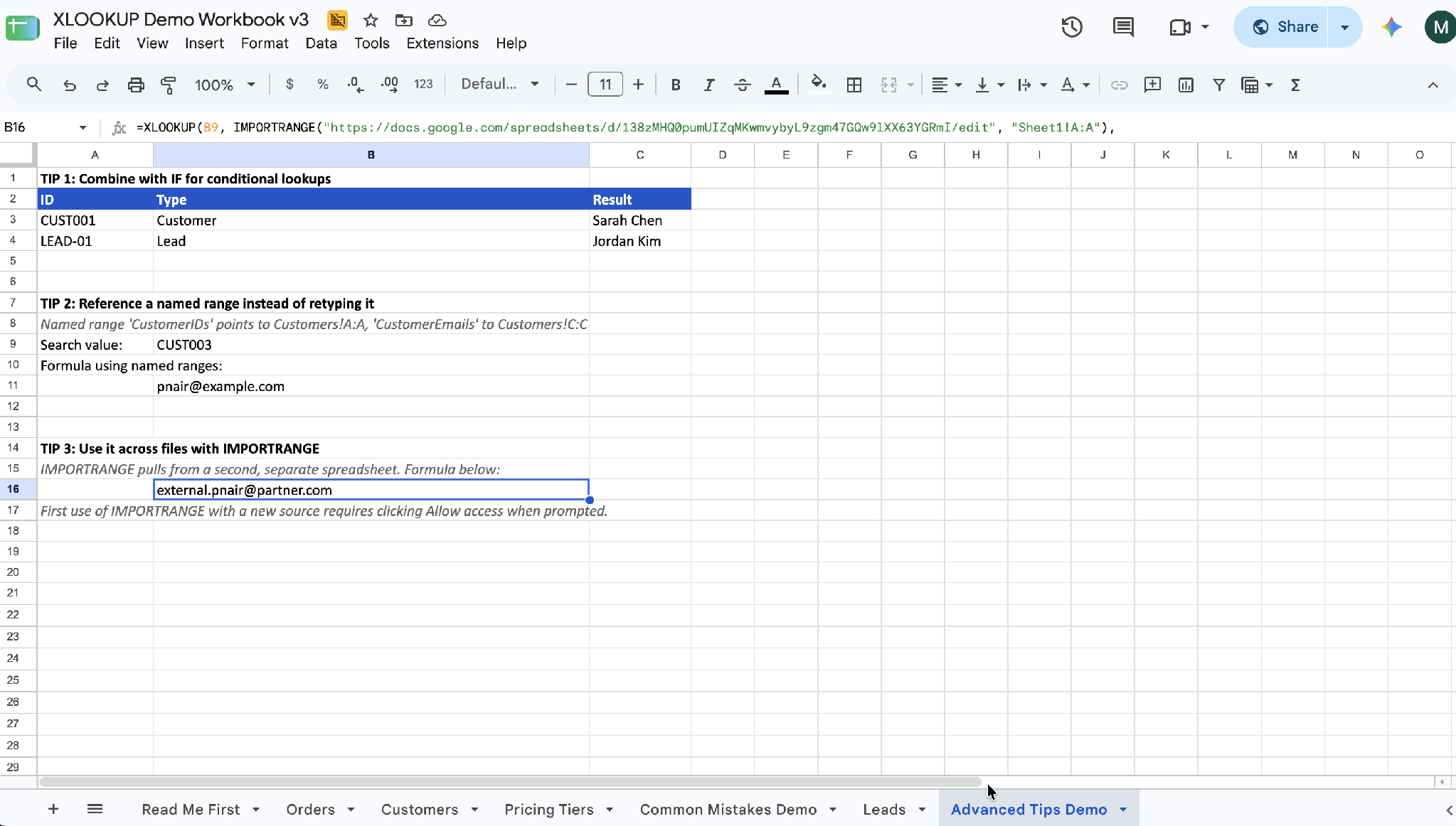
Reference a range instead of retyping it: If several formulas share the same lookup and result ranges, naming those ranges first makes the XLOOKUP formulas easier to read and less error-prone to copy across cells.

Match on two criteria at once: XLOOKUP only takes one search key, so combining two columns into one means joining them with an ampersand on both sides of the comparison. To find a product's price for a specific region, with product names in A2:A7, regions in B2:B7, and prices in C2:C7:
=ARRAYFORMULA(XLOOKUP("Desk Lamp"&"West", A2:A7&B2:B7, C2:C7))
The ARRAYFORMULA wrapper matters here. Without it, the two joined ranges aren't compared row by row, and the formula returns #N/A even when a match exists.
Search across a row instead of a column: XLOOKUP works the same way when the data runs horizontally. With quarter labels in B1:E1 and revenue figures in B2:E2:
=XLOOKUP("Q3", B1:E1, B2:E2)
This returns the revenue figure sitting directly below Q3, the same logic as a column-based lookup, just turned sideways.
Where XLOOKUP in Google Sheets hits its ceiling
XLOOKUP exists to solve one problem. It finds a record in one place and pulls related details from another. That's also, word for word, what a database does by default, using a link between two tables to hold the relationship permanently.
A spreadsheet held together by XLOOKUP formulas works well until the data itself needs restructuring. At that point, every formula pointing at the old range needs checking. This comparison of spreadsheet vs database covers that tradeoff directly.
Zite picks up from there. Your records live in a database that edits like a spreadsheet, and an order links to its customer once and stays linked. You then build whatever you need on top of those records (a dashboard, a customer portal, an order tracker), and everyone on the team works from the same live data.
This roundup of no-code app builders covers other tools built around linked data.
Here's how Zite helps once lookups start doing a database's job:
- Keep the spreadsheet you already have: Connect your Google Sheet and the app stays in sync with it, or import the data into Zite's own database if you'd rather leave the spreadsheet behind.
- Linked records: Connect an order to a customer once, and the customer's email shows up on every order with no formula. Adding or reordering fields doesn't break the link the way it breaks a range reference.
- AI fields: Give a column an instruction, and Zite fills it in for every record, categorizing, summarizing, or scoring each one. No lookup can do that.
- Apps on the same data: A dashboard, a portal, and an internal tool can all run on the same records, and each person sees only what you allow.
- Workflows you can read: Describe what should happen when a record changes and Zite builds the workflow, laid out visually so you can check every step. Start one from a button, from a connected service like Stripe or Slack, or on a schedule (Business plan and up).
- Unlimited users: Every plan includes unlimited users, so sharing with the team doesn't change the bill.
Start building with Zite for free if XLOOKUP in Google Sheets is the only thing holding your data together.
Frequently asked questions
How long does it take to learn XLOOKUP in Google Sheets?
Learning XLOOKUP in Google Sheets takes 3 to 7 minutes for a basic formula, if you already understand what a lookup does. Adding a fallback value, a match mode, or a search direction takes a bit more practice, usually 10 to 15 minutes before it feels natural.
What's the hardest part of using XLOOKUP?
The hardest part of using XLOOKUP is keeping the lookup range and result range the same size and in the right order. A mismatch produces an #N/A error that gives no real explanation. Confirming both ranges cover the same rows before entering the formula avoids most of this.
Is XLOOKUP better than VLOOKUP?
Yes, XLOOKUP is generally the better choice over VLOOKUP, since it can return a result from any column relative to the search value, including ones to the left. It also includes a built-in fallback for missing matches, which VLOOKUP handles only by wrapping the formula in a separate function.
Can XLOOKUP search both vertically and horizontally?
Yes, XLOOKUP can search both vertically and horizontally with the same formula. Point the lookup range at a column for a vertical search, or a row for a horizontal search. XLOOKUP adjusts automatically, without needing a separate function like HLOOKUP.
Can Zite help with XLOOKUP?
Yes, Zite can help with XLOOKUP by removing the need for it entirely. It connects related records directly in a database, so the relationship an XLOOKUP formula recreates each time is already built into the data itself.