
The Google Sheets QUERY function lets you filter, sort, and group data using a SQL-like language. One formula replaces what would otherwise take several nested functions.
I've replaced entire helper-column setups with a single QUERY formula more times than I can count. Once the syntax clicks, it becomes the function you reach for instead of stacking FILTER, SORT, and VLOOKUP together.
Here's the step-by-step, the syntax mistakes that cause a #VALUE! error, and why writing formulas this close to SQL is a sign you're pushing the spreadsheet past what it's built for.
What is the QUERY function?
QUERY runs a database-style query against a range of cells. It uses clauses like SELECT, WHERE, and GROUP BY, borrowed from Google's own query language, not the syntax you'd use elsewhere in a spreadsheet.
It's the closest a spreadsheet gets to acting like a database. Once your sheet has outgrown a simple list, check this spreadsheet vs database breakdown, or this list of Google Sheets alternatives, to decide what changes next.
What you'll need before starting
Prerequisites:
- A Google Sheet with tabular data: consistent columns and one row per record.
- Basic comfort with the idea of filtering or sorting data, even if not with SQL specifically.
- No paid account or add-on required.
Time required: 5 to 10 minutes for a basic query, 15 to 20 minutes to get comfortable with WHERE conditions and GROUP BY.
How to use the QUERY function in Google Sheets: step-by-step
Step 1: Write the basic structure
QUERY takes three arguments. The first is the data range, the second is a query string in quotes, and the third is an optional header-row count.
=QUERY(A1:D100, "SELECT A, B", 1)Swap in SELECT * if you want every column back instead of naming them one by one.
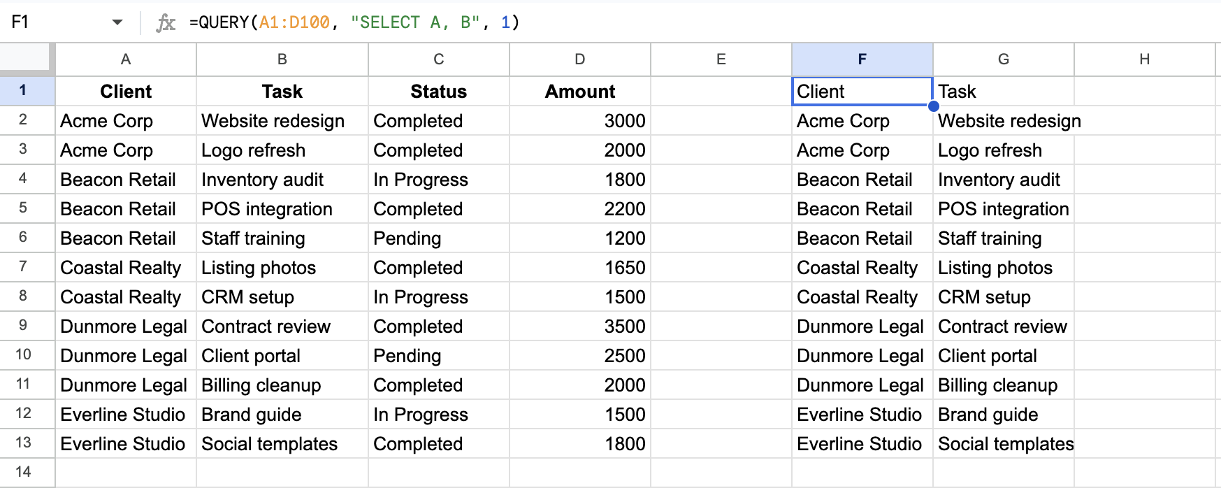
Pro tip: Set the headers argument explicitly to 0, 1, or however many header rows you have. Sheets guesses when it's left out, and the guess is based on what your data looks like, so a wrong guess can leave your header row in the results or hide a row of your data.
Step 2: Select specific columns
Inside the quotes, SELECT chooses which columns to return. For a range on the same sheet, name the columns by their letters, the way Step 1 does. Step 7 covers the Col1, Col2 style you need once the data comes from IMPORTRANGE.
=QUERY(A1:D100, "SELECT A, C", 1)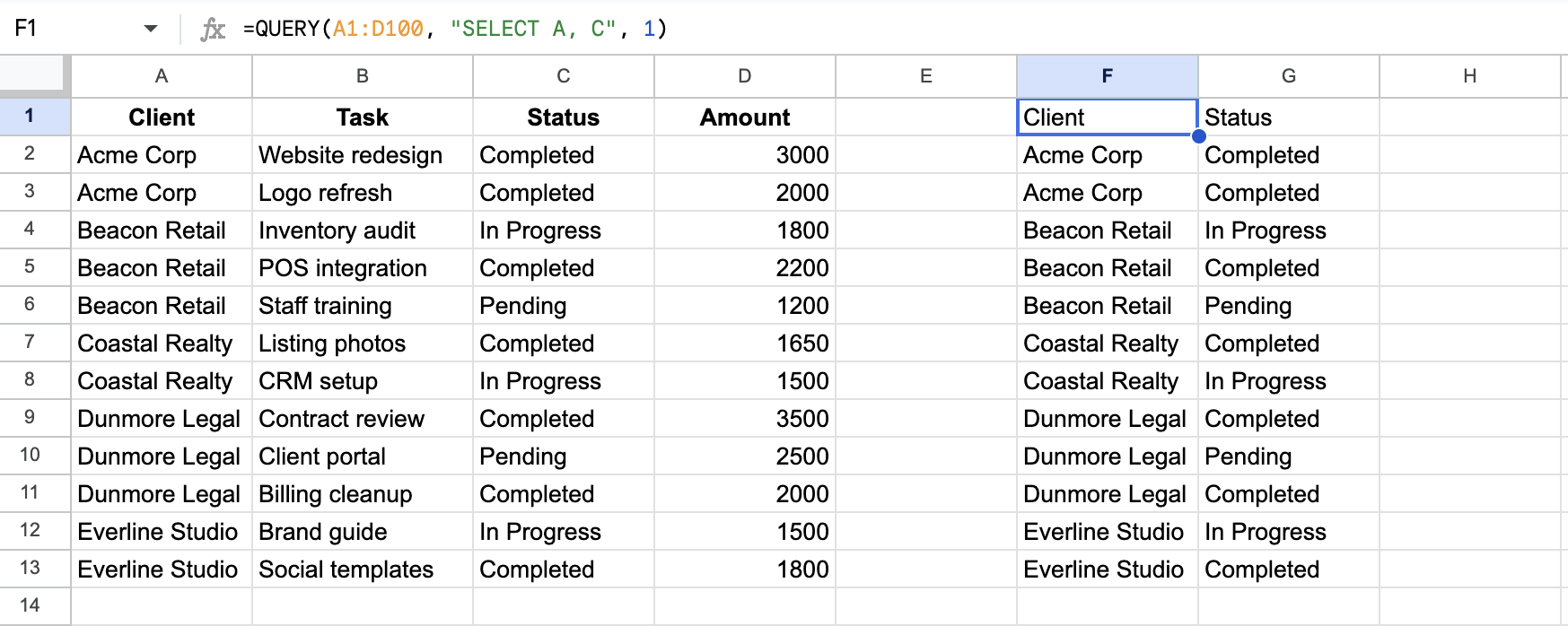
Step 3: Filter rows with WHERE
Add a WHERE clause to return only rows matching a condition. Text values need single quotes; numbers don't.
=QUERY(A1:D100, "SELECT A, B WHERE C = 'Completed'", 1)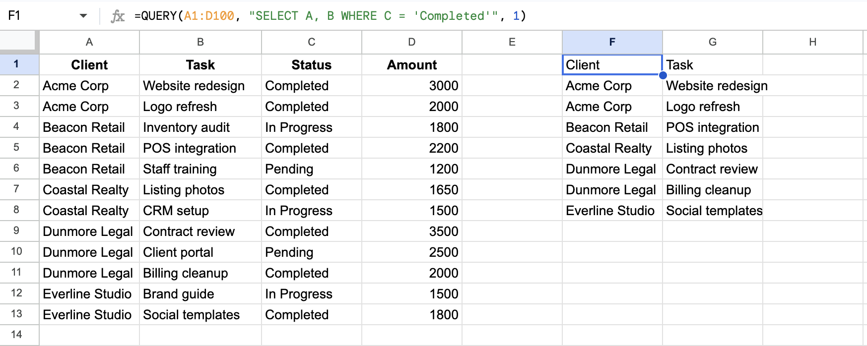
Pro tip: Combine conditions with AND or OR to filter on more than one thing at once, like WHERE C = 'Completed' AND D > 500.
Pro tip: When comparing against a date, use the word date before the value, like WHERE D > date '2026-01-01'. Leaving it out is a common reason a date comparison silently returns nothing.
Step 4: Sort results with ORDER BY
Add ORDER BY to sort the output by one or more columns, with ASC or DESC to control direction.
=QUERY(A1:D100, "SELECT A, B WHERE C = 'Completed' ORDER BY B DESC, A ASC", 1)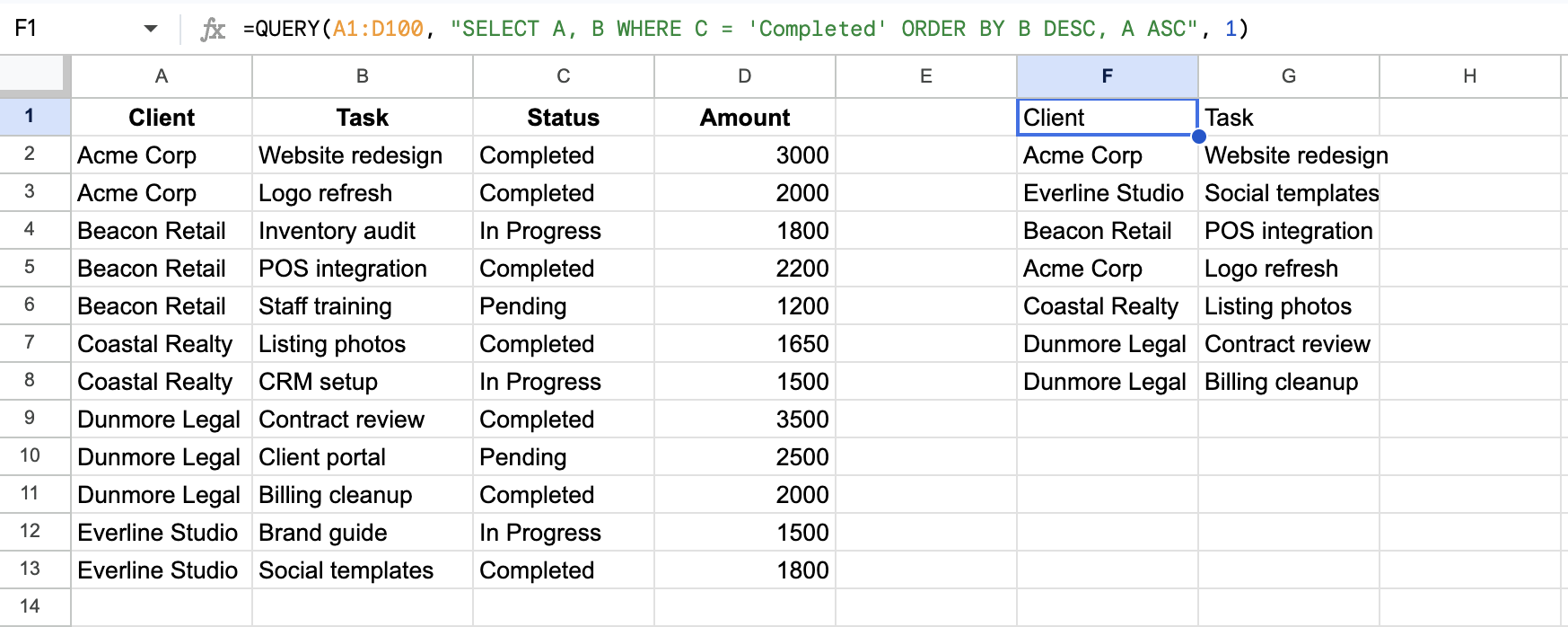
Step 5: Group and summarize with GROUP BY
Use GROUP BY to aggregate data, paired with a summary function such as SUM, COUNT, or AVG in the SELECT clause.
=QUERY(A1:D100, "SELECT A, SUM(D) WHERE A is not null GROUP BY A", 1)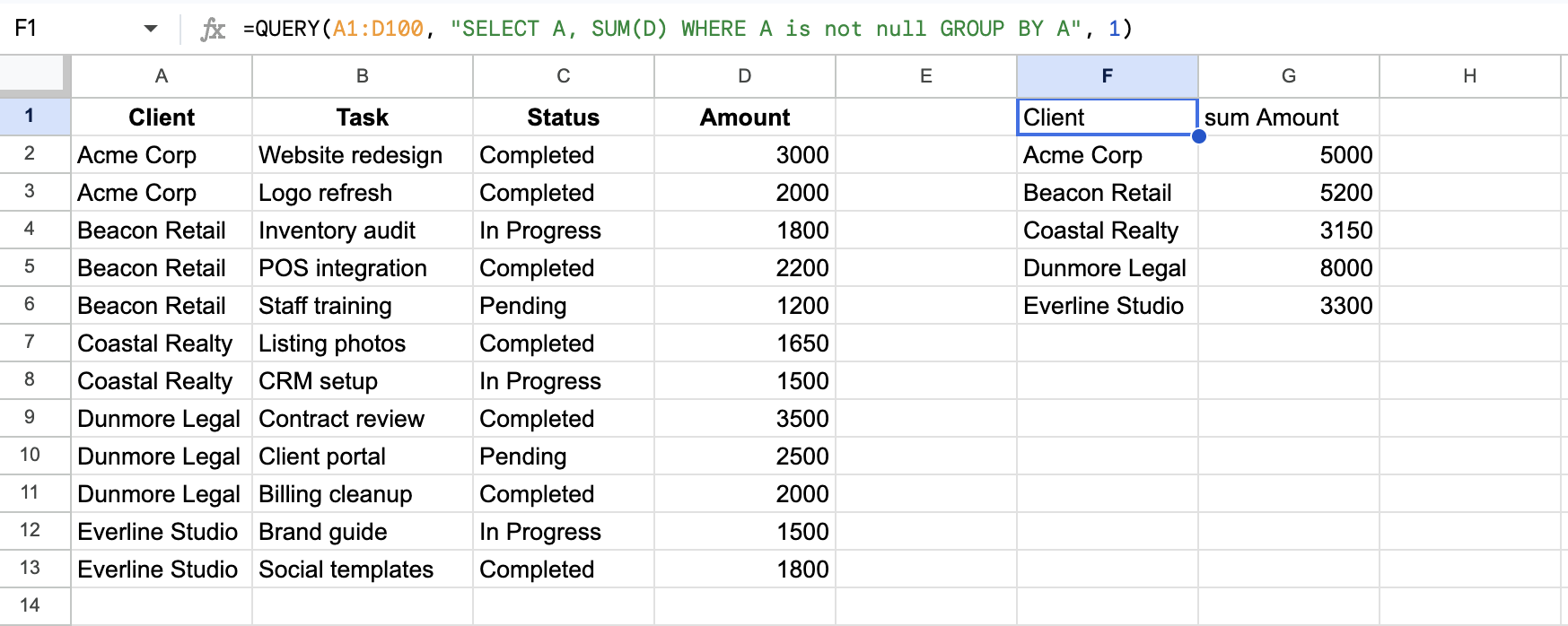
The WHERE A is not null part keeps the empty rows under your data from showing up as a blank group. Leave it out and a blank row appears under the header.
Every column in SELECT needs to either appear in GROUP BY or be wrapped in an aggregation function. Selecting a column that's in neither produces an error. SQL enforces the same rule.
Step 6: Limit or rename the output
Add LIMIT to cap how many rows come back, and LABEL to rename a column in the result instead of showing the default header, such as sum Amount.
I found this out the hard way. QUERY's clauses follow a fixed order: SELECT, WHERE, GROUP BY, PIVOT, ORDER BY, LIMIT, OFFSET, LABEL. Put LABEL before LIMIT, and QUERY throws a #VALUE! error instead of applying either one.
=QUERY(A1:D100, "SELECT A, SUM(D) WHERE A is not null GROUP BY A LIMIT 10 LABEL SUM(D) 'Total'", 1)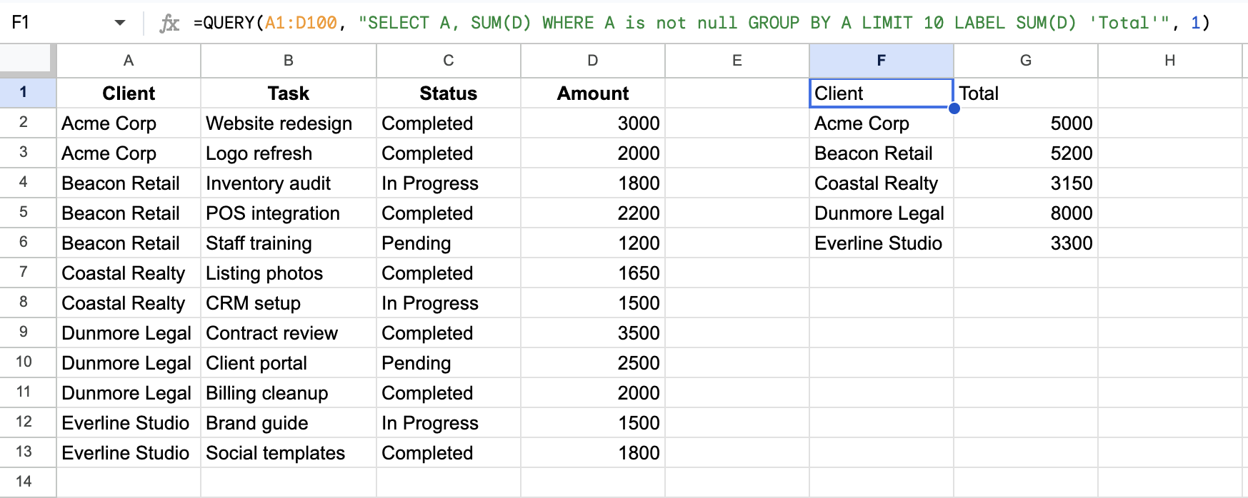
Step 7: Query data from another sheet or file
To pull from a completely separate spreadsheet, wrap IMPORTRANGE in QUERY instead. The source file has to be approved once before it returns anything, so run IMPORTRANGE on its own first and click Allow access when Sheets asks. Column names switch to Col1, Col2 style here, since the data is now an imported array rather than a range on your sheet.
=QUERY(IMPORTRANGE("https://docs.google.com/spreadsheets/d/abcd123abcd123", "Sheet1!A1:D100"), "SELECT Col1, Col2 WHERE Col4 > 1000", 1)
If the imported range starts at column A, Col1 happens to match column A. If it starts partway through the source sheet, such as column C, Col1 refers to column C, not column A.
I've found this mismatch causes more mix-ups than any other part of QUERY's syntax.
This is where QUERY saves a lot of time, since one formula can pull, filter, and reshape data that would otherwise require copying and cleaning it by hand.
Common mistakes to avoid
Small, easy-to-miss details break QUERY's SQL-like syntax. Here's what to check first:
- Mixing up letters and Col numbers: Letters name the sheet's own columns, so they have to fall inside your range. Col numbering applies when the data comes from IMPORTRANGE or an array, and Col1 is the first column of that data, not column A.
- Missing quotes around text values: WHERE C = Completed fails; WHERE C = 'Completed' works. Text needs single quotes; numbers don't.
- Forgetting the date keyword: Comparing a column to a date without the word date in front of it produces no matches instead of an error. Nothing visibly breaks, so it's easy to miss.
- Selecting ungrouped columns with GROUP BY: Every SELECT column needs to be in GROUP BY or wrapped in SUM, COUNT, AVG, or similar, or the query fails.
- Leaving out the headers argument: Omitting it forces Sheets to guess. A wrong guess can duplicate or drop your header row.
Advanced tips
Build a dynamic query from a cell reference. Break out of the quotes to concatenate a cell value into the condition. A dropdown or input cell then controls what the query returns, without editing the formula itself: =QUERY(A1:D100, "SELECT A WHERE C = '"&F1&"'", 1)
Use PIVOT for cross-tabulation in one formula. Adding PIVOT to a query cross-tabulates data like a pivot table, without leaving the formula bar. For a live Airtable dashboard view rather than a static formula result, that is a different job.
Combine QUERY with IMPORTRANGE for cross-file reporting. Wrapping IMPORTRANGE inside QUERY lets you pull and filter data from an entirely different spreadsheet in one step. That combination pays off once you're reporting across multiple files.
Where QUERY signals you're ready for a database
The Google Sheets QUERY function is the point where a spreadsheet starts acting like a database. SELECT, WHERE, and GROUP BY come straight from database language.
If you've written more than a couple of these formulas, you're already thinking in tables and relationships, the way a database does.
Ignoring that pattern just means rebuilding the same workaround again later.
This Sheets vs Airtable comparison covers what changes when data moves into a structure built for it.
Zite gives you that structure from the start: your data lives in a proper database, with the named fields and relationships QUERY was approximating.
For a closer look at what that means in practice, this guide to the best database software is a useful next read.
Here's how Zite helps once QUERY starts feeling like a workaround:
- Keep the spreadsheet you already have: Connect your Google Sheet and Zite keeps the app and the sheet in sync in both directions, or import the data into Zite's own database if you'd rather leave the spreadsheet behind.
- Named fields and linked records: A client record links to its tasks, so "every completed task for Acme" is a filter you set up, not a query string you debug.
- Ask questions instead of writing queries: Connect Zite to ChatGPT or Claude and ask questions about your data in plain language. If you ever want SQL, the same connection can run read-only queries against your tables.
- AI fields: Give a field an instruction, and Zite fills it in for every record, whether that means summarizing, categorizing, or scoring. That goes beyond anything a QUERY clause can do.
- One live source for the whole team: Everyone works from the same records, so an update by one person is what everyone else sees. The Team plan adds roles and granular permissions, so you can control who can use and edit what.
- Unlimited users: Every plan includes unlimited users, so sharing views with a team doesn't change the bill.
If the Google Sheets QUERY function has started doing a database's job without a database underneath it, Zite is free to try.
Frequently asked questions
How long does it take to learn the QUERY function?
Writing a basic SELECT query takes 5 to 10 minutes if you're already comfortable with the idea of filtering data. Getting fluent with WHERE conditions, GROUP BY, and combining QUERY with IMPORTRANGE takes closer to 15 to 20 minutes of practice. The clauses read like SQL, even though the syntax underneath is Google's own.
What's the hardest part of using QUERY in Google Sheets?
The hardest part is choosing between letters and Col numbers, since letters follow the sheet's own columns, while Col1, Col2 numbering applies when the data comes from IMPORTRANGE or an array and counts from wherever that data starts. From what I've seen, that gap trips people up more than the SQL-like syntax itself.
Do I need to know SQL to use QUERY?
No. Familiarity with SQL concepts like SELECT, WHERE, and GROUP BY makes QUERY much faster to learn, since the clause names carry straight over. Without that background, expect to look up clause syntax more often at first. Start with SELECT and WHERE from Steps 2 and 3, then add GROUP BY once those feel familiar.
What if my QUERY formula returns a #VALUE! error?
A #VALUE! error from QUERY almost always comes from one of three things. Look for missing quotes around WHERE text values, a SELECT column that's neither grouped nor wrapped in an aggregation function, or clauses written out of order. A headers argument that doesn't match your range is a different problem: it won't throw an error; it just duplicates or drops a row.
What's the difference between QUERY and VLOOKUP?
VLOOKUP returns a single value from one matching row. QUERY returns an entire table, filtered, sorted, or grouped however you specify, and it updates automatically as the data changes.