
A pivot table in Google Sheets summarizes a large set of rows into totals, counts, and averages, grouped however you want to see them. It does this without writing a single formula.
I've built dozens of them for reporting and cleanup work. Once the row-versus-column layout clicks, manually summing filtered ranges stops making sense.
Here's how to create a pivot table in Google Sheets, step by step. You'll also see the mistakes that produce a table full of zeros or blanks, and what to reach for once rebuilding for every new question gets old.
What is a pivot table?
A pivot table takes rows of raw data, like a list of transactions, and reorganizes them into a summary. Think total sales by region, count of orders by status, or average time by category. You choose what to group by and what to calculate, and Sheets does the math.
The reason it beats formulas for this job is flexibility. Changing what you're summarizing, from totals by month to totals by product, is dragging a field to a different box, not rewriting a SUMIF.
This assumes your source data is already clean rows and columns. If it's outgrown that shape, this spreadsheet vs database breakdown covers what to do about it.
What you'll need before starting
Prerequisites:
- A Google Sheet with tabular data: consistent column headers and one row per record.
- No blank rows or columns inside the data range.
- No paid account or add-on required.
Time required: 2 to 5 minutes for a basic pivot table, 10 to 15 minutes if you're adding filters and calculated fields.
How to create a pivot table in Google Sheets: step-by-step
Step 1: Select your data range
Click anywhere inside your data, or select the full range including headers. Sheets uses the header row to name the fields you'll drag into the pivot table next.
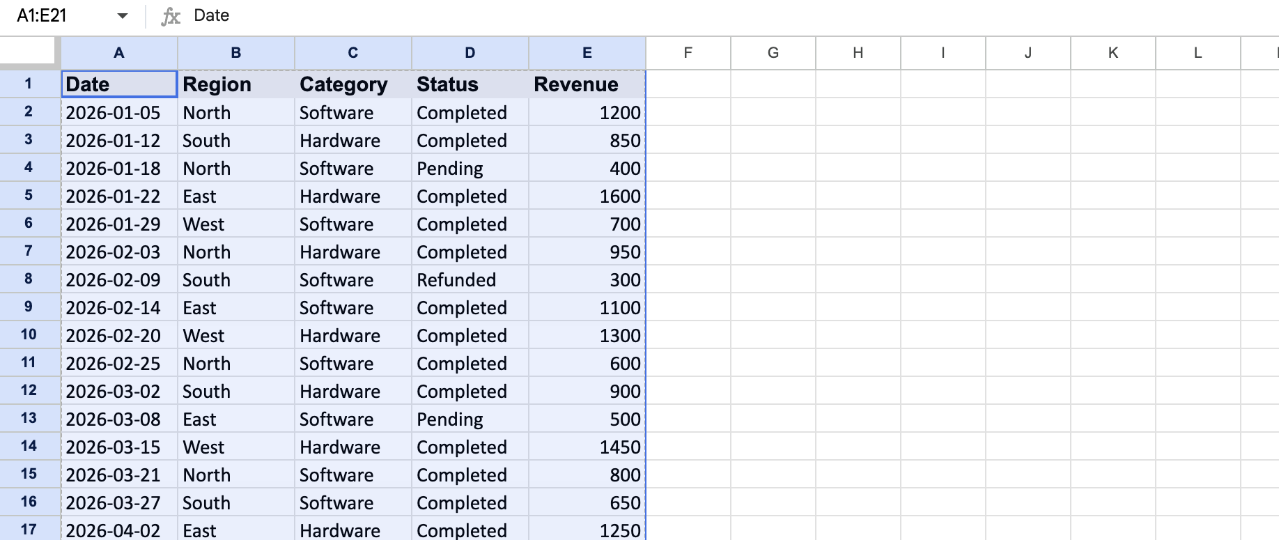
Pro tip: Clicking a single cell inside a clean, contiguous table usually works fine, since Sheets auto-detects the full range. Select the range manually if your data has any gaps.
Step 2: Insert the pivot table
Go to Insert > Pivot table. Sheets asks where to place it, either a new sheet or a location in the current one.
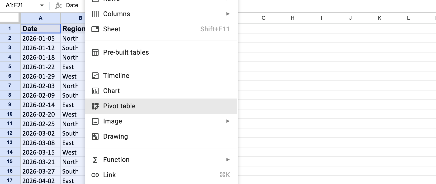
A new sheet is the safer default, since it keeps the summary separate from your source data.
Step 3: Add a row field
In the pivot table editor, click Add next to Rows, then choose the field you want to group by, such as Region or Product Category. Each unique value becomes its own row in the summary.
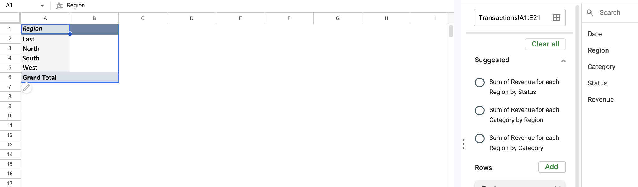
This is the field that answers "grouped by what?" Start with the grouping that matters most to the question you're answering.
Step 4: Add a values field
Click Add next to Values and choose the field you want to calculate, like Revenue or Order Count. Sheets defaults to SUM, but you can change it to COUNT, AVERAGE, MIN, MAX, and several other summary types.
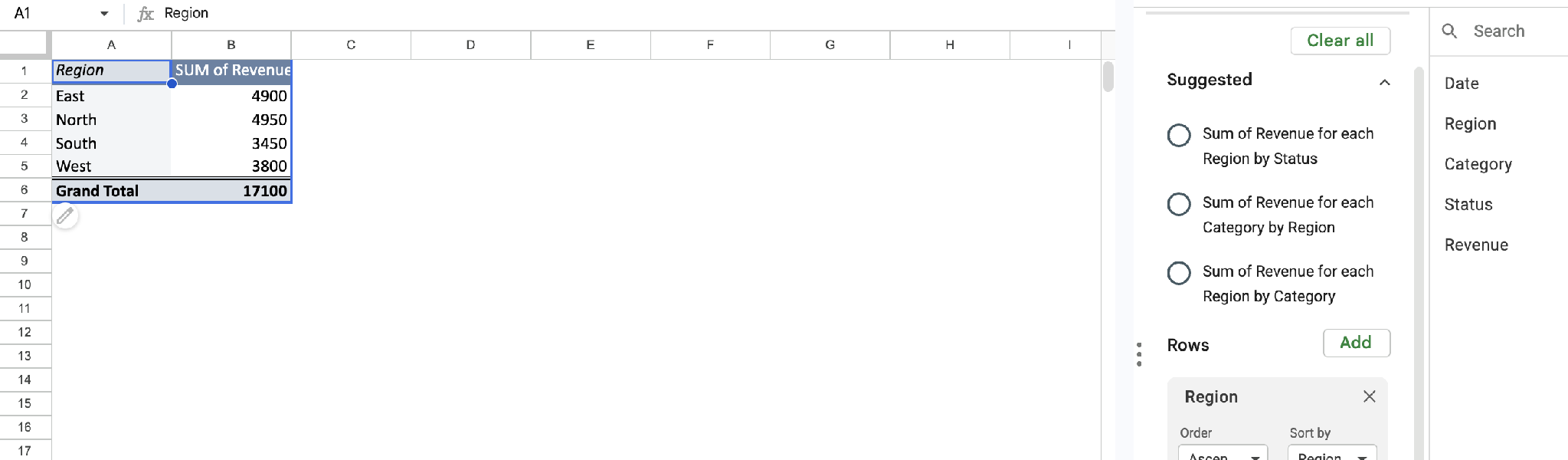
Pro tip: If your values column shows all zeros, the field is probably formatted as text. Check the source data's formatting before assuming the pivot table is broken.
Step 5: Add a column field to compare two things at once
If you want to compare a metric across two dimensions at once, like revenue by region and by month, click Add next to Columns. Choose the second field there. This turns a simple list into a grid you can read in both directions.
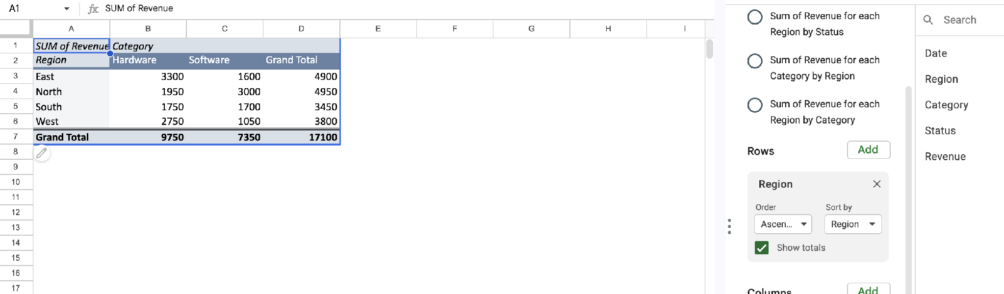
Skip this step if one grouping already answers your question. Adding a column field you don't need makes the table wider and harder to read.
Step 6: Add filters to narrow the data
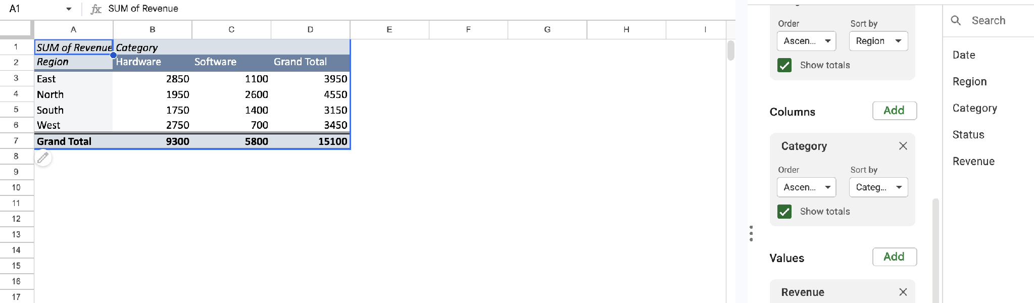
Click Add next to Filters to restrict the summary to a subset, like only completed orders or only this year's transactions. Filters change what feeds the pivot table without touching your source data.
One catch: if you filter by value and then add new source data, you have to update the filter before that data shows up.
Step 7: Update the range when you add new rows
Edits to existing rows in your data range update the pivot table automatically. New rows are the catch, and it depends on how you set the range.
A whole-column range like A:C picks them up automatically. A bounded range like A1:C50, which is what you get from clicking a single cell, stops at row 50 until you widen it with Select data range in the editor.
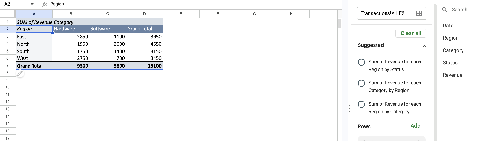
This step is easy to miss, since a pivot table that looks current can leave out your newest data.
Can I create a pivot table in Google Sheets with Gemini?
Yes, if you have Gemini access. Open the side panel from Ask Gemini in the top right, then describe what you want, like "create a pivot table showing total sales by region." Gemini builds the table and shows a preview card. You click Apply to confirm, or adjust the prompt if the rows, columns, or summary aren't what you meant.
The catch is availability. Gemini in Sheets needs an eligible Google Workspace plan on a work or school account, or a Google AI plan (Google AI Pro) on a personal account. It's not part of the free Sheets you use for the manual method above.
Can I build a pivot table from data on more than one sheet?
Not directly. A pivot table pulls from one contiguous range, so you have to combine data split across tabs first.
The QUERY function does this by stacking ranges: =QUERY({Sheet1!A1:C; Sheet2!A1:C}, "SELECT * WHERE Col1 IS NOT NULL"). Curly braces stack the two ranges on top of each other into one combined result, which becomes your pivot table's source. Match the column structure across sheets first, since QUERY combines by position, not by header name.
Common mistakes to avoid
A pivot table can look broken when the real issue is how the source data was set up. Here's what to check first:
- Missing or inconsistent headers: A pivot table names its fields from your header row, and Google requires one on every column. Leave a header blank, and that column has nothing to be selected by. Duplicates make fields impossible to tell apart.
- Blank rows or columns inside the range: A gap in your data can shorten the detected range, leaving rows out of the summary.
- Text-formatted numbers: Values stored as text won't sum correctly, producing a table full of zeros instead of an error that would be easier to catch.
- Forgetting to expand the range: A bounded range stops where you set it, so new rows below it never reach the summary. Setting the range to whole columns avoids this.
- Over-adding fields: Stacking several row and column fields at once often results in a table that's too dense to read. Start narrow and add fields only as the question requires them.
Sometimes the data itself has outgrown a spreadsheet, and no amount of cleanup fixes it. This list of Google Sheets alternatives is worth a look.
Advanced tips
Once the basic pivot table works, a few extra moves make it noticeably more useful. Here's where to start:
- Group dates automatically: Right-click a date cell inside the pivot table itself, then choose Create pivot date group and pick a period like month, quarter, or year. That turns a long list of dates into a readable trend.
- Use calculated fields for custom metrics: Add a calculated field to compute something not in your raw data, like a custom ratio. That skips adding a helper column to the source sheet. For a percentage of total, you don't need one, since that's a built-in option under Values.
Does Google Sheets have a pivot chart?
Yes. Select a pivot table, then insert a chart from it; the chart stays in sync as the underlying data changes. That's the closest a pivot table gets to a lightweight dashboard on its own, without rebuilding it manually every time the numbers move.
For a fuller version of that idea, this guide to Airtable dashboards covers how to build them, where they run out of room, and what to use instead.
Where pivot tables hit their ceiling
A pivot table answers one question well at a time. Ask a different question, and you're often rebuilding the layout. That's fine for occasional reporting, but it becomes real friction when several people want to check different numbers on their own schedule.
That's the gap between a report and a dashboard. If your team keeps rebuilding the same pivot table with slightly different fields for different people, a live view built once and shared is usually the better fix.
This breakdown of custom dashboard software covers what that looks like beyond a spreadsheet.
Zite starts a layer lower, with the data itself. Your records live in a real database, so everyone works from the same live data. When someone updates a record, every view of it is current.
Describe the view you want, and Zite generates a first draft in minutes. This AI dashboard guide walks through the process.
Here's how Zite helps once a pivot table needs constant rebuilding:
- Keep the spreadsheet you already have: Connect your Google Sheet and the dashboard stays in sync with it, or import the data into Zite's own database if you'd rather leave the spreadsheet behind.
- A live view instead of a static summary: The dashboard automatically reflects current data. Nobody has to reopen it and refresh the numbers.
- Built on a real database: Records sit in linked tables with defined fields, editable like a spreadsheet. Fields have a set type, so a number can't end up stored as text and a blank row can't cut the data short, which are the two things that break a pivot table.
- Shareable without rebuilding per person: Each person logs in and sees only the records you allow, so one dashboard serves the whole team without a copy for every request.
- Unlimited users: Every plan includes unlimited users, so sharing the dashboard with a whole team doesn't change the bill.
Start building with Zite for free if you're rebuilding the same pivot table in Google Sheets more often than you'd like.
Frequently asked questions
How long does it take to create a pivot table in Google Sheets?
Creating a basic pivot table takes 2 to 5 minutes. Select your data, insert the pivot table, and add a row and a values field. Adding filters, a column field, or calculated metrics for a more detailed summary takes closer to 10 to 15 minutes.
What's the hardest part of creating a pivot table?
The hardest part is preparing clean source data. Blank rows, inconsistent headers, or numbers stored as text all produce a pivot table that looks broken. The problem is upstream, in how the data was entered.
Do I need a paid Google account to use pivot tables?
No, pivot tables are a standard Google Sheets feature available on any free Google account. There's no premium tier or add-on required.
Can Zite help me build something like a pivot table?
Zite builds a live dashboard from your data in minutes. That covers the same "summarize this by that" job a pivot table does, without rebuilding it each time the question changes. It's a different kind of tool, working from a real database rather than inside a spreadsheet.
What if my pivot table shows blank or zero values?
Blank or zero values almost always come from numbers stored as text, blank rows inside the data range, or new rows added outside the pivot table's original range. In my experience, the pivot table itself is rarely the problem.