

=INDEX(return_range, MATCH(lookup_value, lookup_range, 0))That is the INDEX MATCH Google Sheets formula. MATCH finds which row holds your value, and INDEX returns the cell from that row in any column you choose, to the left or right of the lookup column.
I ran the sample formulas below in a live Google Sheet, and the results shown come from that sheet.
Below are a worked example, a drop-down lookup, MATCH search types, wildcards, a VLOOKUP comparison, multiple criteria, lookups across tabs and files, and fixes for #N/A, #NUM!, and #REF! errors.
What is INDEX MATCH?
INDEX MATCH pairs two functions, INDEX and MATCH, and each part of the formula does one job.
Here are the three parts of the formula:
-
INDEX(return_range, row): Returns the cell at that row position of the range you want back, such as a price column.
-
MATCH(lookup_value, lookup_range, 0): Returns the position of the lookup value within the lookup range, such as the row where a product name sits.
-
The 0: Asks MATCH for an exact match. Google's MATCH page says the default of 1 assumes the range is sorted in ascending order, and 0 is required when it isn't.
Google's INDEX page adds that setting the row or column number to 0 returns the whole column or row.
In my test, =INDEX(A2:D5, 0, 3) on the product table below returned all four prices, and =INDEX(A2:D5, 3, 0) returned the whole Mug row. Leave the cells next to the formula empty so the results can spill into them.

What you'll need before starting
Here are three things to have ready:
-
A Google Sheet with a header row and your data in columns.
-
A lookup column with unique values, since MATCH returns the first match it finds.
-
Basic comfort with cell references such as B2:B5.
Time required: About five minutes for the basic formula, plus 15 minutes for multiple criteria and lookups across files.
How to use INDEX MATCH in Google Sheets: Step-by-step
The steps below use a small product table, and every result shown comes from this data.
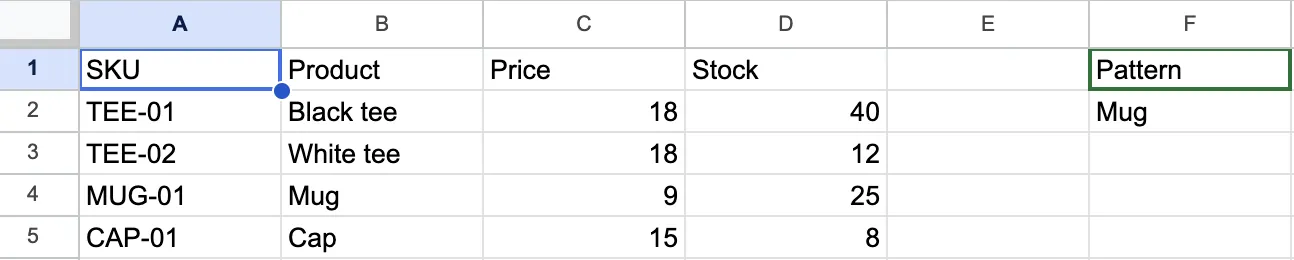
Here is the product table in A1:D5:
| SKU | Product | Price | Stock |
|---|---|---|---|
| TEE-01 | Black tee | 18 | 40 |
| TEE-02 | White tee | 18 | 12 |
| MUG-01 | Mug | 9 | 25 |
| CAP-01 | Cap | 15 | 8 |
Step 1: Set up the data and a lookup cell
Enter the table in A1:D5, then type the product you want to find in cell F2, such as Mug. The formula will read F2, so you can change the product without editing the formula.
Step 2: Test MATCH on its own
Type =MATCH(F2, B2:B5, 0) in G2. MATCH returns 3 because Mug is the third item in B2:B5. Seeing that number first confirms the lookup works before you add INDEX.
Step 3: Wrap MATCH in INDEX
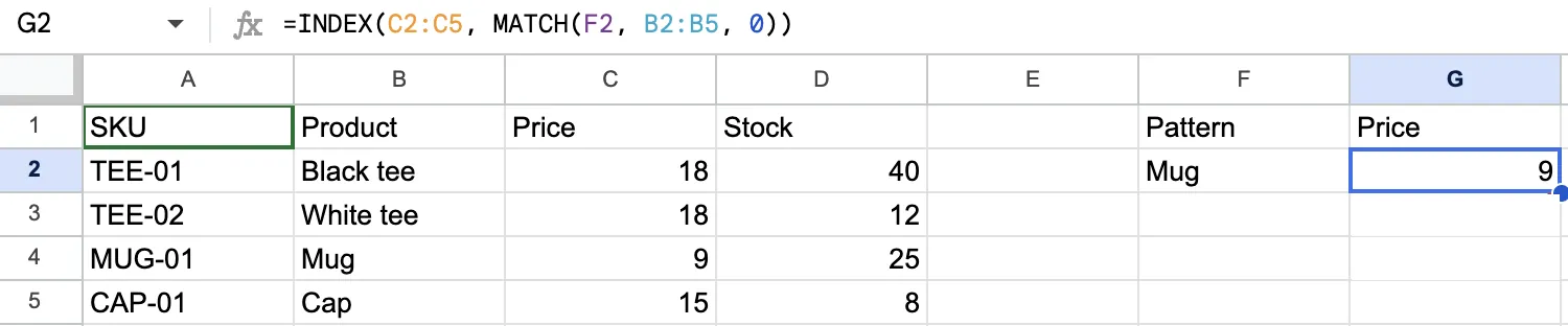
Replace the formula in G2 with this one.
=INDEX(C2:C5, MATCH(F2, B2:B5, 0))MATCH returns 3, and INDEX returns the third cell of C2:C5, so G2 shows 9, the price of a mug.
Pro tip: Start both ranges on the same row. A mismatch returns a neighboring row's value with no error, as the fix for misaligned ranges below shows.
Step 4: Lock the ranges and fill down
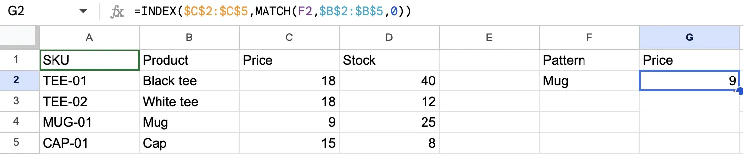
Add dollar signs so the ranges don't slide when you copy the formula to other rows.
=INDEX($C$2:$C$5, MATCH(F2, $B$2:$B$5, 0))List more products in F3 and F4, then drag the formula down. Without the dollar signs, the ranges move down one row with each copy.
Step 5: Look to the left
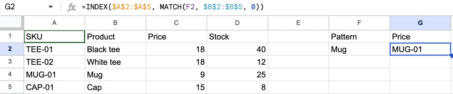
Unlike VLOOKUP, INDEX MATCH can return a column to the left of the lookup column. To return the SKU for the product in F2, point INDEX at column A.
=INDEX($A$2:$A$5, MATCH(F2, $B$2:$B$5, 0))For Mug, it returns MUG-01. Google's INDEX page says VLOOKUP can only be used when the lookup value is to the left of the value you want back.
Step 6: Handle products that are not found
Wrap the formula in IFERROR so a missing product shows a message.
=IFERROR(INDEX($C$2:$C$5, MATCH(F3, $B$2:$B$5, 0)), "Not found")With Scarf in F3, the formula returns Not found.
Google's IFERROR page says IFERROR(exp1, exp2) is logically equivalent to IF(NOT(ISERROR(exp1)), exp1, exp2), so it catches every error type. A broken range also shows Not found, so add IFERROR last, after the formula works.
Build a lookup with a drop-down list
A drop-down in the lookup cell replaces typing, so the product name always matches the table.
Here are the three steps to set it up:
1. Select F2, then open Data > Data validation > Add rule.
2. Under Criteria, choose Dropdown from a range, then select B2:B5 as the list and click Done.
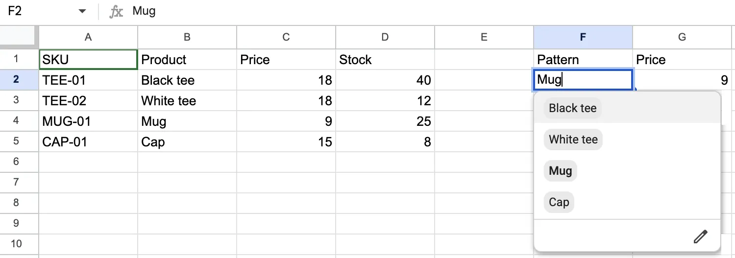
3. Pick a product from the arrow in F2, and the Step 4 formula in G2 updates.
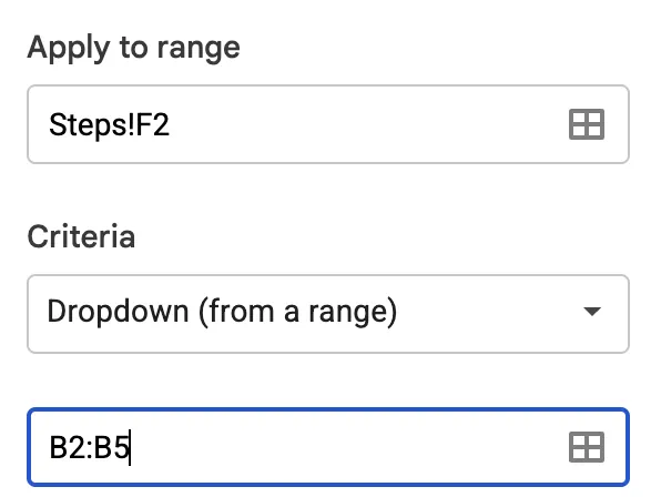
Google's drop-down help page says the list updates when the source range changes, and that entries not on the list are rejected by default. Choosing Cap returns 15.
MATCH search types: Exact, ascending, and descending
The third argument of MATCH controls how it searches. Google's MATCH page defines three values.
Here are the three search types:
-
0: Exact match, and required when the range is not sorted.
-
1 (default): Assumes the range is sorted in ascending order and returns the largest value less than or equal to the lookup value.
-
-1: Assumes the range is sorted in descending order and returns the smallest value greater than or equal to the lookup value.
Ascending bands with search type 1
Search type 1 suits lookups against thresholds, such as a commission rate that rises with sales. This table sits in A1:B5, with sales from 0 up.
| Sales from | Rate |
|---|---|
| 0 | 0% |
| 500 | 2% |
| 1000 | 5% |
| 5000 | 8% |
With 1200 in D2, this formula returns 5%, because 1000 is the largest threshold at or below 1200.
=INDEX(B2:B5, MATCH(D2, A2:A5, 1))In my test, 5000 returned 8%, and 499 returned 0%. A value below the first threshold, such as -5, returned #N/A. Searching 1200 with search type 0 also returned #N/A, because no row holds exactly 1200.

Descending limits with search type -1
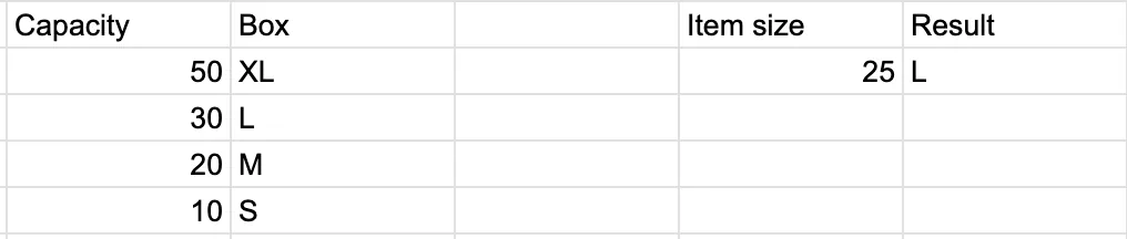
Search type -1 finds the smallest value that is still large enough. This table lists box capacities from largest to smallest in H1:I5.
| Capacity | Box |
|---|---|
| 50 | XL |
| 30 | L |
| 20 | M |
| 10 | S |
With an item size of 25 in K2, this formula returns L, because 30 is the smallest capacity at or above 25.
=INDEX(I2:I5, MATCH(K2, H2:H5, -1))In my test, a size of 5 returned S and a size of 60 returned #N/A, because no box is that large.
INDEX MATCH with wildcards for partial matches
When you only know the start or end of a name, add a wildcard to the lookup value. Google's MATCH page doesn't mention wildcards, but they worked in my test with search type 0.
The product table is in A1:D5, and the pattern sits in F2.
=INDEX($C$2:$C$5, MATCH(F2, $B$2:$B$5, 0))Here are the patterns I tested:
-
Start of a name: Mu* uses the asterisk for any number of characters, so it matches Mug and returns 9.
-
One unknown letter: M?g uses the question mark for exactly one character, so it also matches Mug and returns 9.
-
End of a name: *p matches any name ending in p, so it matches Cap and returns 15.
To search by what a user types, join the asterisk to the cell, as in MATCH(F2&"*", $B$2:$B$5, 0). With Ca in F2, that returns 15. Without the asterisk, Mu and Ca return #N/A, because no product has exactly that name.

INDEX MATCH vs VLOOKUP
INDEX MATCH has two advantages over VLOOKUP, and both come from how the formulas point at data.
Here is how the two formulas compare:
| Feature | VLOOKUP | INDEX MATCH |
|---|---|---|
| Looks left of the lookup column | No | Yes |
| Column reference | A number you type | The range itself |
| After you insert a column | Can return the wrong column | Adjusts automatically |
| Formula length | Shorter | Longer |
Google's INDEX page labels VLOOKUP's search key and column index as hardcoded, while INDEX MATCH can make the row and the column dynamic.
Ablebits explains that VLOOKUP needs the column order number, so adding a column can return the wrong value, while INDEX MATCH uses cell references that Sheets adjusts for you.
Sheets also has XLOOKUP, which can return a column to the left of the lookup column. INDEX MATCH is still worth learning because you will meet it in spreadsheets other people built.
INDEX MATCH MATCH: A two-way lookup
A second MATCH lets INDEX find both the row and the column.
Here is the sales table by region and quarter:
| Region | Q1 | Q2 | Q3 | Q4 |
|---|---|---|---|---|
| North | 120 | 135 | 150 | 170 |
| South | 90 | 95 | 110 | 125 |
| East | 140 | 150 | 145 | 160 |
With the table in A1:E4, South in G1, and Q3 in G2, this formula returns 110.
=INDEX(B2:E4, MATCH(G1, A2:A4, 0), MATCH(G2, B1:E1, 0))The first MATCH finds the row for South, and the second finds the column for Q3 in the header row. The same pattern appears on Google's INDEX page, where both the row number and the column number are dynamic.

INDEX MATCH with multiple criteria
Some rows need two columns to tell them apart. In this price list, each product comes in several sizes, so a lookup needs both.
Here is the price list by product and size:
| Product | Size | Price |
|---|---|---|
| Tee | S | 18 |
| Tee | M | 18 |
| Tee | L | 20 |
| Hoodie | S | 40 |
| Hoodie | M | 40 |
| Hoodie | L | 44 |
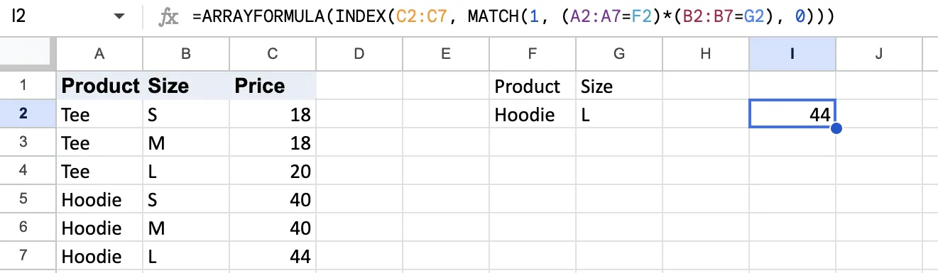
With the list in A1:C7, Hoodie in F2, and L in G2, there are two ways to find the price.
Multiply the conditions
Each comparison checks every row and returns TRUE or FALSE. TRUE times TRUE equals 1, so the result is 1 only on the row that meets both conditions.
=ARRAYFORMULA(INDEX(C2:C7, MATCH(1, (A2:A7=F2)*(B2:B7=G2), 0)))MATCH finds the first 1, and INDEX returns that row's price, which is 44. To add a third condition, multiply by one more comparison. ARRAYFORMULA lets the comparisons run across the whole range.
Join the columns into one key
Combine the criteria into one search key and match it against the combined columns.
=ARRAYFORMULA(INDEX(C2:C7, MATCH(F2&"|"&G2, A2:A7&"|"&B2:B7, 0)))The vertical bar keeps different pairs from producing the same key. Without it, "A1" and "B" would join into the same text as "A" and "1B". This formula also returns 44.
Pro tip: Turn the criteria cells into drop-down lists with Data > Data validation, so a typo can't cause a #N/A.
Both methods return only the first matching row. To list every match, use FILTER.
INDEX MATCH across sheets and files
Another tab in the same file
Put the tab name and an exclamation mark before each range, and use single quotes if the name has spaces.
=INDEX(Prices!C2:C7, MATCH(A2, Prices!A2:A7, 0))With Hoodie in A2, this formula returns 40, the price on the first Hoodie row.
If the INDEX range and the MATCH range start on different rows or cover a different number of rows, the formula reads the price from the wrong product.
Another file with IMPORTRANGE
Replace each range with an IMPORTRANGE call that points at the other file. Bounded ranges keep the two imports the same size.
=INDEX(IMPORTRANGE("https://docs.google.com/spreadsheets/d/YOUR_SPREADSHEET_ID/edit", "Prices!C2:C1000"), MATCH(A2, IMPORTRANGE("https://docs.google.com/spreadsheets/d/YOUR_SPREADSHEET_ID/edit", "Prices!A2:A1000"), 0))The first time, Sheets shows a #REF! error with an Allow access button if you own the source file, according to Google's IMPORTRANGE page. Click it once for the file. If someone else owns it, request access and wait for the owner to grant it.
For a lookup you need repeatedly, import the range into a spare tab once and run INDEX MATCH against that tab. The formulas stay short, and the file makes one import.
How to fix INDEX MATCH errors
These six problems each produce an error or a wrong value.
#N/A because the value is not found
When MATCH finds no match, it returns #N/A, and the INDEX around it shows the same error. OWOX lists a trailing space, a number stored as text, and a different spelling as the usual causes.
If F4 holds "Mug " with a trailing space, the formula returns #N/A. Wrapping the lookup value in TRIM fixes it.
=INDEX($C$2:$C$5, MATCH(TRIM(F4), $B$2:$B$5, 0))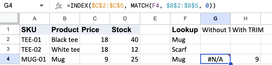
#N/A because MATCH has a two-dimensional range
Google's MATCH page says the range must be one-dimensional, and a range with both height and width greater than 1 returns #N/A. Use a single column such as B2:B5 for the lookup range.
A wrong value from ranges that do not line up
If MATCH searches B1:B5 while INDEX reads C2:C5, the position is off by one, and Mug returns 15, the price of the cap below it.
No error appears, so the wrong price looks correct until you check it. Make both ranges begin on one row and share a height.
#NUM! because the position is outside the range
In my test, =INDEX(C2:C5, 9) on a four-row range returned #NUM!. The row number, 9, is larger than the four rows in the range. Size the INDEX range so it includes every row number the formula can ask for.
Results that change when you copy the formula
If G2 is correct but G3 and G4 show the wrong prices, the ranges shifted as you copied the formula. Add the dollar signs from Step 4.
#REF! because the formula sits inside its own range
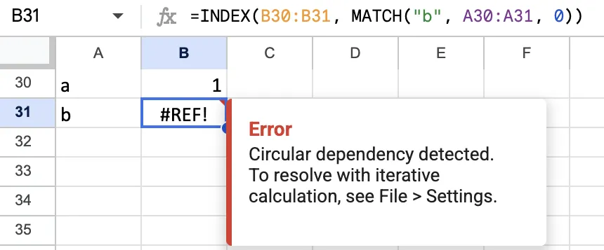
In my test, a formula in B31 that read =INDEX(B30:B31, MATCH("b", A30:A31, 0)) returned #REF! with the message "Circular dependency detected," because its range included its own cell. Move the formula outside the range it reads, or shorten the range so it stops above the formula.
Common mistakes to avoid
Here are three mistakes to avoid:
-
Leaving out the 0: Without it, MATCH treats the list as sorted and can land on the wrong product. In my test on the unsorted sample table, Mug then returned 15, the price of the cap.
-
Expecting every match: INDEX MATCH returns the first matching row only, so use FILTER when a value appears more than once.
-
Adding IFERROR too early: IFERROR turns every error into your message, including a broken range, so add it last, after the formula returns the right value.
Advanced tip: A case-sensitive lookup
MATCH ignores letter case. To tell "Hoodie" from "hoodie", match on EXACT instead.
=ARRAYFORMULA(INDEX(C2:C7, MATCH(TRUE, EXACT(F2, A2:A7), 0)))For Hoodie in F2, this formula returns 40. For hoodie, it returns #N/A because no row matches that exact case.
When INDEX MATCH stops being the answer
INDEX MATCH suits a lookup inside one workbook. Here are four signs the data has outgrown it:
-
Lookups across many tabs: Every extra tab adds ranges that must start on the same row and span the same rows.
-
Files chained by IMPORTRANGE: Google warns that chains cause delays and advises limiting the number of receiving sheets.
-
Duplicate keys: INDEX MATCH stops at the first match, so a repeated SKU returns only one row.
-
Several editors: When several people edit at once, conflicts creep in, and that is one sign a spreadsheet has been outgrown. This spreadsheet vs database guide covers the other signs.
A database avoids these problems by storing each fact once and linking records. This guide to Google Sheets alternatives covers tools with linked tables built in, and this roundup of no-code app builders shows the tools that make the move.
Zite replaces lookup formulas with linked records
Once your data lives in linked tables, Zite removes the need for lookup formulas, and this Sheets vs Airtable comparison shows where each tool fits.
Here are four ways Zite covers what INDEX MATCH does:
-
Linked records: A linked record is a relationship between records in different tables, such as an order linked to a customer, so no MATCH formula has to find it.
-
Lookup fields: A lookup field shows information from a linked record, such as the customer's email on each order.
-
Rollups: A rollup field turns the values in linked records into one result, using functions such as SUM, AVERAGE, or COUNT.
-
Import your sheet: You can import data from Google Sheets, CSV, Excel, or Airtable, up to 250,000 records at once, and importing from Google Sheets doesn't change your spreadsheet.
Zite can also build apps on top of those tables, so your team no longer has to work in the sheet itself. Each person gets an app for their part of the job, such as an order form for sales or a stock screen for the warehouse, and you describe which records each person should see. That eases the "several editors" problem above too, since nobody has to sort or overwrite a shared range.
Zite's free plan includes unlimited users and 5,000 records, so you can import a copy of your sheet and test linked records before changing anything.
Frequently asked questions
Is INDEX MATCH better than VLOOKUP in Google Sheets?
Yes, INDEX MATCH is better than VLOOKUP in Google Sheets when the value you want sits left of the lookup column or the columns may change. Google's INDEX page says VLOOKUP can only be used when the lookup value is to the left of the value you want back. Sheets also offers XLOOKUP, which can return a column to the left.
Can INDEX MATCH return more than one match?
No, INDEX MATCH can't return more than one match, because MATCH stops at the first hit and INDEX returns a single cell. To return every row that matches, use FILTER, which lists all rows that meet a condition. On the sample price list, INDEX MATCH returns the first Hoodie price only, while FILTER lists every Hoodie row.
How do you use INDEX MATCH with multiple criteria in Google Sheets?
You use INDEX MATCH with multiple criteria in Google Sheets by multiplying the conditions inside MATCH, or by joining the criteria columns into one key, and wrapping the formula in ARRAYFORMULA. Both versions return 44 for a Hoodie in size L on the sample price list, and both return only the first matching row.
What if INDEX MATCH returns #N/A?
INDEX MATCH returns #N/A in Google Sheets when MATCH can't find the lookup value or is given a two-dimensional range. Check for trailing spaces and text-versus-number mismatches, wrap the lookup value in TRIM if needed, and make sure the lookup range is a single column. A misspelled lookup value returns #N/A too.
Can Zite help me with INDEX MATCH?
Zite can help with INDEX MATCH lookups once your data lives in linked tables, using linked records and lookup fields in place of matching formulas. Importing a sheet copies its data into Zite, so the original sheet stays as it was. Zite also builds apps on those tables, so each person works in their own view. This list of AppSheet alternatives covers other ways to turn a sheet into an app.