

VLOOKUP in Google Sheets searches down the first column of a range for a value, then returns data from a column to its right. That's why it's the classic first lookup formula to learn. I've used it for years. The mistakes that trip people up are almost always the same two or three, no matter how well someone understands what it's for.
Here's the step-by-step, plus the setup that has to be right before you write the formula. At the end, the mistake that returns a wrong answer with nothing to flag it is leaving out FALSE, which lets VLOOKUP settle for a close-enough match.
What is VLOOKUP?
VLOOKUP looks for a value in the leftmost column of a range and returns a value from another column in that same row. The return column is counted by position from the left edge of the range.
The name is short for "vertical lookup," since it searches down a column instead of across a row.
One rule matters more than the rest: your search value has to sit in the leftmost column of whatever range you point VLOOKUP at, because VLOOKUP can't look to its own left.
What you'll need before starting
Prerequisites:
- A Google Sheet with two ranges you want to match up.
- A second sheet or range to pull matching data from, if you're looking up across sheets.
- No paid account or add-on required.
Time required: 3 to 5 minutes for a basic lookup, 10 minutes if you're adding error handling or working across sheets.
How to use VLOOKUP in Google Sheets: step-by-step
These six steps take you from a blank formula to a working lookup, in the order you'll type them.
Step 1: Arrange your data with the search column on the left
Before writing the formula, confirm the value you'll search for sits in the leftmost column of the range you plan to use. If a customer ID is what you're looking up, it needs to be the first column in that table. The data you want returned sits somewhere to its right.
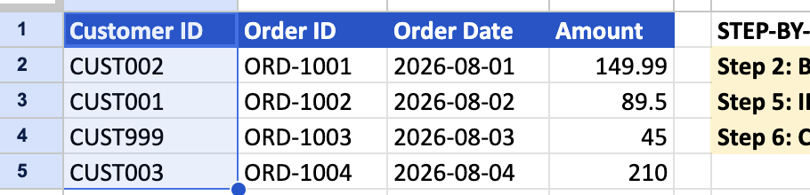
Pro tip: If the value you need to search by isn't in the leftmost column of your existing data, that's the point where VLOOKUP stops being the right tool. INDEX/MATCH or XLOOKUP solves that specific problem instead.
Step 2: Write the basic VLOOKUP formula
The syntax is:
=VLOOKUP(search_key, range, index, is_sorted)
To look up a customer ID in A2 against a table in Sheet2 spanning columns A through D, returning the value from the third column of that range:
=VLOOKUP(A2, Sheet2!A:D, 3, FALSE)

Step 3: Count the index number from the left edge of the range
The index argument is a column number counted from 1, starting at the leftmost column of the range you specified. If your range is B:E, column B is 1, C is 2, D is 3, and E is 4, regardless of the sheet's actual column letters.
Pro tip: Counting from the range instead of from column A is easy to get backward. Recheck the index number any time you change which columns the range covers.

Step 4: Set exact match with FALSE
The fourth argument controls whether VLOOKUP requires an exact match. Setting it to FALSE requires an exact match and returns an error if none exists. Leaving the fourth argument out, or setting it to TRUE, allows an approximate match instead, which requires the first column of the range to be sorted in ascending order.
For almost everything outside of numeric range lookups (like matching a score to a grade band), FALSE is what you want.

Step 5: Handle a missing match with IFERROR
VLOOKUP has no built-in fallback for a missing match, unlike newer lookup functions. Wrap it in IFERROR to show something readable instead of a raw #N/A.
One caution: IFERROR hides every error, not just a missing match. If a changed column breaks your index number later, you'll see "Not found" instead of the error that would have warned you.
IFNA catches only the missing match and leaves the rest visible:
=IFNA(VLOOKUP(A2, Sheet2!A:D, 3, FALSE), "Not found")

Step 6: Reference another sheet the same way
Point VLOOKUP at a range on a different sheet by prefixing the range with the sheet name, exactly as in the examples above. The mechanics don't change, only where the data lives.

Common mistakes to avoid
Here are the six setup issues worth checking first:
- Leaving out FALSE for an exact match: This is the classic VLOOKUP mistake. Without it, the formula defaults to an approximate match and can return a plausible-looking wrong answer instead of an error, which is easy to miss.
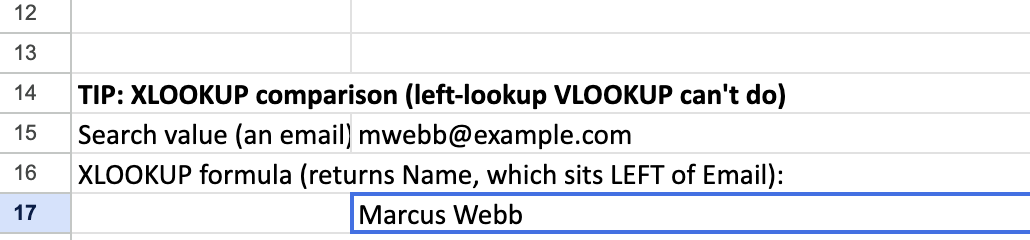
- The search value isn't in the leftmost column: VLOOKUP can't look to its left. If the value you need to search by sits to the right of the data you want, the formula won't work no matter how the index is set.
- The index number breaks after inserting a column: The index is a hard count, and it doesn't update automatically when columns move. Adding or removing a column inside the range changes what that number points to. That's the same fragility that makes a full Google Sheets alternative worth a look once this kind of breakage becomes routine.
- Mismatched data types: A search value stored as a number won't match a lookup column storing the same value as text, and the reverse is also true.
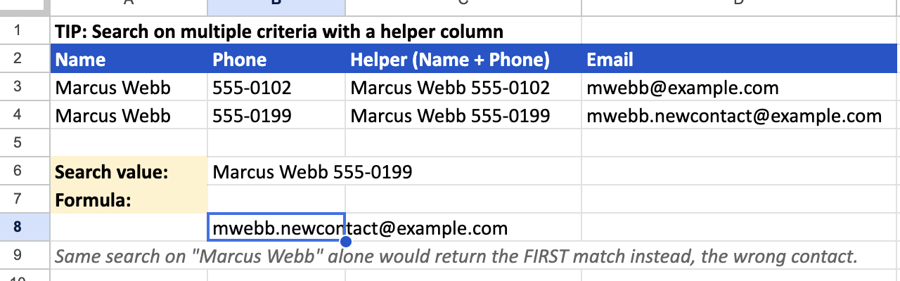
- Assuming VLOOKUP returns every match: If your search value appears more than once in the lookup column, VLOOKUP only returns the first match it finds. Duplicate search values need a workaround, like the helper column covered below.
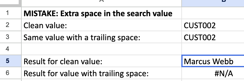
- Extra spaces in the search value or lookup data: An invisible trailing space can make an otherwise identical value fail to match.
What the error on your screen means:
A mismatched data type, an extra space, or a search value outside the leftmost column all produce the same result: #N/A, meaning VLOOKUP searched the whole range and found nothing that matched.
#REF!, sometimes shown with the fuller text "VLOOKUP evaluates to an out of bounds range," means the index number points past the last column in your range, usually because a column got added or removed after the formula was written.
Leaving out FALSE doesn't throw an error. It returns an answer that looks correct, which is what makes it the mistake worth checking for first.
Advanced VLOOKUP tips in Google Sheets
Use an open-ended range for growing data: A range like Sheet2!A:D covers every row in those columns, including ones added later. You won't need to update the formula as the source data grows.
Use a wildcard for a partial match: Set the fourth argument to FALSE, then use an asterisk in the search key to match any text around it. "*cake*" finds a product with "cake" anywhere in its name.

Search on multiple criteria with a helper column: VLOOKUP takes only one search value, so a helper column that joins two columns lets you match on both at once. Build it in the source table as the leftmost column of your range, using an ampersand:
=B2&" "&C2
Then build the same combined value on the search side and point VLOOKUP at that:
=VLOOKUP(E2&" "&F2, Sheet2!A:D, 4, FALSE)
Combine with IF for conditional lookups: Wrapping VLOOKUP inside an IF statement lets you check one table under one condition and a different table otherwise.

Pull from a separate spreadsheet with IMPORTRANGE: VLOOKUP only searches within one spreadsheet on its own. Put IMPORTRANGE inside the VLOOKUP, in place of the range, to search a table that lives in a different file:
=VLOOKUP(A2, IMPORTRANGE("spreadsheet_url", "Sheet1!A:D"), 3, FALSE)
The first time you point to a new source file, Sheets shows a #REF! error until you click Allow Access. Leaning on this a lot is a sign it might be time to weigh Sheets vs Airtable for the whole workflow. If you're pulling several sheets together just to build one view, a dedicated view like Airtable dashboards is worth comparing too.

Consider INDEX/MATCH or XLOOKUP once you hit the leftmost-column wall: If you keep needing to look up a value that sits to the right of what you want returned, that's the specific problem XLOOKUP was built to solve. No restructuring of your data required.
Where VLOOKUP shows the ceiling of a spreadsheet
VLOOKUP works because your data holds a specific shape, with the search column on the left and the result a fixed number of columns over. That same shape is also VLOOKUP's biggest weak point. Insert a column, reorder the sheet, or add a field, and a formula that worked yesterday can return the wrong answer today with no warning.
Nothing in the formula tracks what the data means, only where it sits.
A database relationship doesn't have this problem, since two records stay connected by what they are, independent of where either one sits in a grid. This comparison of spreadsheet vs database covers that difference in more depth.
Zite picks up from there. Your records live in a database that edits like a spreadsheet, and a customer links to their orders once and stays linked, whatever gets added or reordered around them. You then build whatever you need on top of those records (a dashboard, a customer portal, an order tracker), and everyone on the team works from the same live data.
Here's how Zite helps once lookup formulas get fragile:
- Keep the spreadsheet you already have: Connect your Google Sheet and the app stays in sync with it, or import the data into Zite's own database if you'd rather leave the spreadsheet behind.
- Linked records: Connect an order to a customer once, and the customer's details show up on every order with no formula and no index number to recount. Adding or reordering fields doesn't break the link the way it breaks a range reference.
- AI fields: Give a column an instruction, and Zite fills it in for every record, categorizing, summarizing, or scoring each one. No lookup can do that.
- Apps on the same data: A dashboard, a portal, and an internal tool can all run on the same records, and each person sees only what you allow.
- Workflows you can read: Describe what should happen when a record changes and Zite builds the workflow, laid out visually so you can check every step. Start one from a button, from a connected service like Stripe or Slack, or on a schedule (Business plan and up).
- Unlimited users: Every plan includes unlimited users, so sharing with the team doesn't change the bill.
Start building with Zite for free if VLOOKUP in Google Sheets breaks more often than it works.
If the underlying data itself has outgrown a spreadsheet, this guide to AI database software covers that wider question.
Frequently asked questions
How long does it take to learn VLOOKUP in Google Sheets?
Learning VLOOKUP in Google Sheets takes a few minutes for a basic formula, once your data is arranged with the search column on the left. The part that takes longer to stick is the leftmost-column rule itself, since it runs opposite to how newer functions like INDEX/MATCH or XLOOKUP work.
What's the most common VLOOKUP mistake?
The most common VLOOKUP mistake is leaving out FALSE as the fourth argument, which lets the formula default to an approximate match. That default can return a plausible-looking wrong answer instead of a clear error. A wrong result can sit in a sheet for a long time before anyone catches it.
Why can't VLOOKUP look to the left?
VLOOKUP can't look to the left because it's built to search only the leftmost column of a range and return a value from a column to its right. That direction is fixed in how the function works. INDEX/MATCH and XLOOKUP both solve this by letting the result live in any column relative to the search value.
What's the difference between VLOOKUP and HLOOKUP?
VLOOKUP searches vertically, down the first column of a range, while HLOOKUP searches horizontally, across the first row. Use HLOOKUP when your data is organized in rows instead of columns, with related values reading left to right instead of top to bottom.
Can Zite help with VLOOKUP?
Yes, Zite can help with VLOOKUP by removing the need for it entirely. It connects related records directly in a database, so the relationship a VLOOKUP formula rebuilds every time is already part of the data.